> For the complete documentation index, see [llms.txt](https://anufrievroman.gitbook.io/freepaths/llms.txt). Markdown versions of documentation pages are available by appending `.md` to page URLs; this page is available as [Markdown](https://anufrievroman.gitbook.io/freepaths/basic-tutorials/nanowire.md).

# Nanowire

The example input file `examples/nanowire.py`, located in the [examples](https://github.com/anufrievroman/freepaths/tree/master/examples) folder, shows thermal transport simulation in a simple nanowire at room temperature. Let's run this input file as:

```
freepaths nanowire.py
```

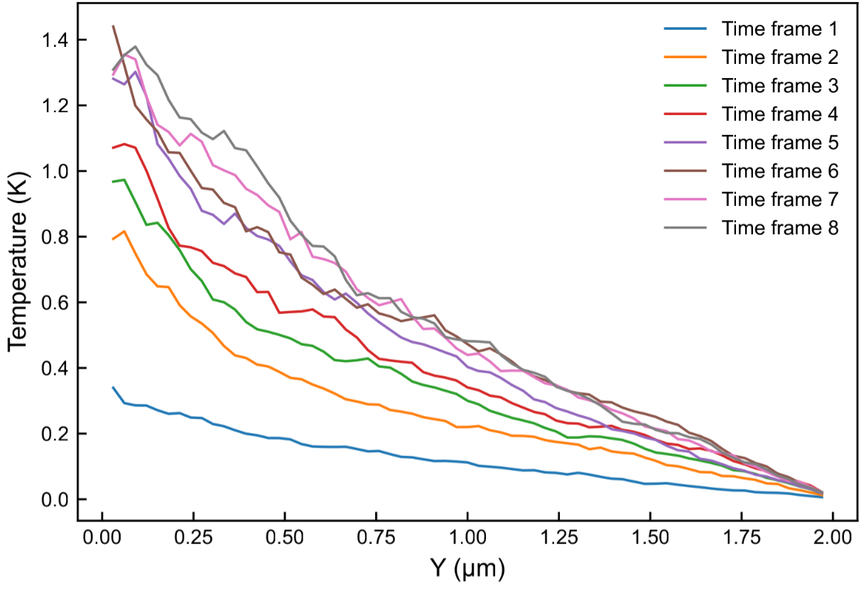
After the simulation, we can see the output files in the Results folder. For example, phonon paths in such a structure showing mostly diffusive behavior:

<figure><img src="/files/0chFpglDZgwWKtQ19vt6" alt=""><figcaption><p>Example of phonon paths in the structure.</p></figcaption></figure>

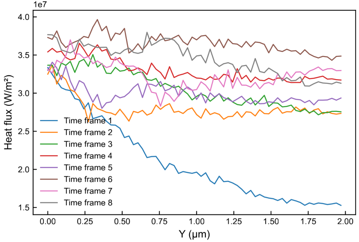
Also, the algorithm calculates the thermal profiles, heat flux, and the thermal conductivity at different time intervals. From the profile plots, we can see how the temperature profiles converge after about the 6th timeframe, as the system is reaching the steady state:

<figure><img src="/files/eAYt10hVx8k0a6ynU0TP" alt="" width="563"><figcaption><p>Temperature profiles at different time intervals.</p></figcaption></figure>

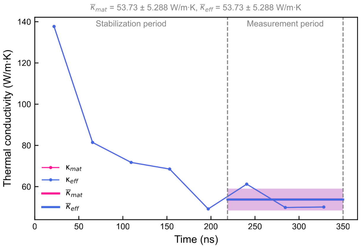
Likewise, the heat flux converges to the flat line in the last few time frames:

<figure><img src="/files/l4ytY5BZNIwJzwqU7gFb" alt="" width="563"><figcaption><p>Heat flux profiles converge to the flat line in the steady state.</p></figcaption></figure>

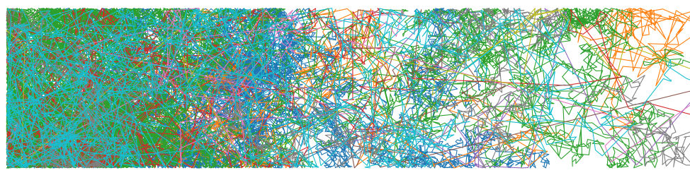
This can be used to estimate the [thermal conductivity](/freepaths/theory/themal-conductivity-calculation.md) of the structure via the Fourier law. The plot of thermal conductivity shows the convergence and the averaging in the steady state interval:

<figure><img src="/files/aQxVMqiSvvofR9iB40QX" alt="" width="563"><figcaption><p>Thermal conductivity convergence and averaging over the steady state period.</p></figcaption></figure>

For a simple nanowire, the [material and effective](/freepaths/theory/themal-conductivity-calculation.md#effective-vs-material-thermal-conductivity) thermal conductivities are identical and equal to about 29 W/m·K, which is consistent with experimental observations. Note that this short (200 nm) domain shows strong ballistic suppression compared to bulk silicon; conductivity rises toward the bulk value for longer wires.

Now, we can try another approach to the [thermal conductivity calculation](/freepaths/theory/themal-conductivity-calculation.md#mean-free-path-approach). We take the same input file but reduce the number of phonons to 30 and run it with `-s` flag:

```
freepaths -s nanowire.py
```

The program calculates [the integral over the phonon branches](/freepaths/theory/themal-conductivity-calculation.md#mean-free-path-approach), and we obtain a comparable value of the thermal conductivity of about 38 W/m·K. The two methods need not match exactly here: MFP sampling captures the cross-section-limited scattering strength but not the additional ballistic suppression that the Fourier approach picks up at this short domain length.

## Tips for thermal conductivity calculations

* The software can currently only calculate the thermal conductivity in the y direction. Also, make sure that the phonons are generated at the edge of the simulation domain.
* The software does not give correct results if pillars are present in the simulation.
* Because the calculation relies on the pixel grid to calculate the profiles, make sure that pixels are small enough and maps look good (some discontinuities in the pixels adjacent to holes are expected and correct).
* Simulate enough phonons (> 5000) to get valid results.
* Ensure that [time parameters](/freepaths/getting-started/config-file-creation-guide.md#simulation-time-parameters) are set correctly.